Updates to the XGBoost GPU algorithms
It has been one and a half years since our last article announcing the first ever GPU accelerated gradient boosting algorithm. GPU algorithms in XGBoost have been in continuous development over this time, adding new features, faster algorithms (much much faster), and improvements to usability. This blog post accompanies the paper XGBoost: Scalable GPU Accelerated Learning [1] and describes some of these improvements.
Histogram based tree construction algorithms
Decision tree construction algorithms typically work by recursively partitioning a set of training instances into smaller and smaller subsets in feature space. These partitions are found by searching over the training instances to find a decision rule that optimises for the training objective. While still effectively linear time these algorithms are slow because searching for the decision rule at the current level requires passing over every training instance. The algorithm can be made considerably faster through discretization of the input features.
Our primary decision tree construction algorithm is now a histogram based method such as that used in [2],[3]. This means that we find quantiles over the input feature space and discretize our training examples into this space. Gradients from the training examples at each boosting iteration can then be summed into histogram ‘bins’ according to the now discrete features. Finding optimal splits for a decision tree then reduces to the simpler problem of searching over histogram bins in a discrete space.
The end result of this is a significantly faster and more memory efficient algorithm that still retains its accuracy.
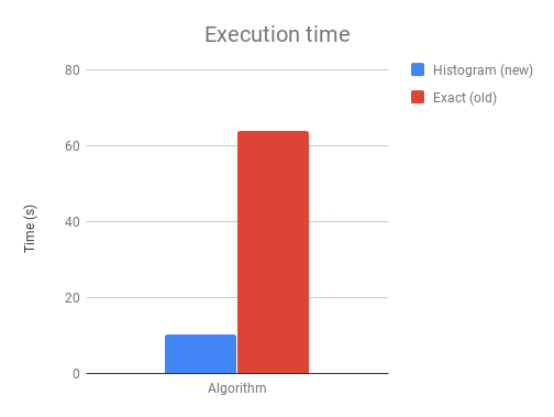
The above chart shows the difference in execution time on a 1M*50 binary classification problem with 500 boosting iterations.
Multi-GPU support
Our histogram algorithm has full multi-GPU support using the NCCL library for scalable communication between GPUs. This means we can do things like run XGBoost on an AWS P3 instance with eight GPUs. The below chart shows the runtime on the 115M row airline dataset as we increase the number of GPUs:
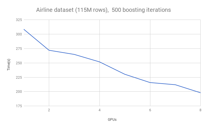
Because of the efficient AllReduce communication primitives, communication throughput is constant as the number of GPUs is increased. Communication costs are also invariant to the number of training examples because only summary histogram statistics are shared. The data set is evenly distributed between GPUs. This allows us to scale up to datasets that cannot fit on a single GPU and use the full device memory capacity of multi-GPU systems.
Data compression
Our current algorithm is also much more memory efficient than the original algorithm published in [4]. This is achieved largely through data compression of the input matrix after discretization. For example, if we use 256 histogram bins per feature and 50 features, there are only 256*50 unique feature values in the entire input matrix. By using bit compression we can store each matrix element using only log2(256*50)=14 bits per matrix element in a sparse CSR format. For comparison, a naive CSR storage format would typically cost a minimum of 64 bits per matrix element.
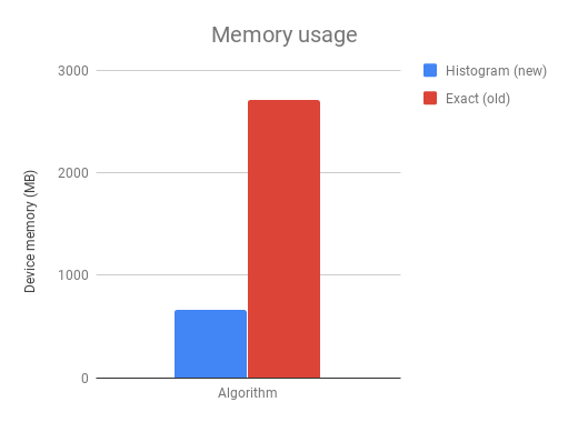
The above chart shows the device memory requirements for a 1M*50 binary classification problem on the histogram algorithm and the exact algorithm.
GPU prediction and gradient calculation algorithms
Traditionally, tree construction algorithms account for most of the time spent in a gradient boosting algorithm. This changed after we developed significantly faster tree algorithms and other parts of the gradient boosting process began to create bottlenecks.
Prediction occurs every iteration in gradient boosting in order to calculate the gradients (residuals) for the next iteration. Users may also want to monitor performance on a test or validation set. This adds up to a large amount of computation on the CPU. We map this computation to a GPU kernel for a performance improvement of between 5-10x in prediction time. Note that this improvement is for memory that is already stored on the GPU. When used for an unseen dataset, prediction algorithms will be slower due to the time taken to copy the matrix to the GPU (i.e. these prediction algorithms are designed for training but not deployment of models).
We also introduce GPU accelerated objective function calculation for some tasks. These can be enabled by setting the objective function as one of:
"gpu:reg:linear", "gpu:reg:logistic", "gpu:binary:logistic", gpu:binary:logitraw"
Moving more parts of the gradient boosting pipeline onto the device removes computational bottlenecks as well as reducing the need to copy memory back and forth between the CPU and GPU across the limited bandwidth PCIe bus. Eventually we hope to move the entire pipeline to the device.
Benchmarking against other GBM algorithms
Below are some benchmarks against other gradient boosting algorithms on an 8 GPU cloud computing instance. Instructions for reproducing these benchmarks can be found here.
| YearPrediction | Synthetic | Higgs | Cover Type | Bosch | Airline | |||||||
|---|---|---|---|---|---|---|---|---|---|---|---|---|
| Time(s) | RMSE | Time(s) | RMSE | Time(s) | Accuracy | Time(s) | Accuracy | Time(s) | Accuracy | Time(s) | Accuracy | |
| xgb-cpu-hist | 216.71 | 8.8794 | 580.72 | 13.6105 | 509.29 | 74.74 | 3532.26 | 89.2 | 810.36 | 99.45 | 1948.26 | 74.94 |
| xgb-gpu-hist | 30.39 | 8.8799 | 43.14 | 13.4606 | 38.41 | 74.75 | 107.70 | 89.34 | 27.97 | 99.44 | 110.29 | 74.95 |
| lightgbm-cpu | 30.82 | 8.8777 | 463.79 | 13.585 | 330.25 | 74.74 | 186.27 | 89.28 | 162.29 | 99.44 | 916.04 | 75.05 |
| lightgbm-gpu | 25.39 | 8.8777 | 576.67 | 13.585 | 725.91 | 74.7 | 383.03 | 89.26 | 409.93 | 99.44 | 614.74 | 74.99 |
| cat-cpu | 39.93 | 8.9933 | 426.31 | 9.387 | 393.21 | 74.06 | 306.17 | 85.14 | 255.72 | 99.44 | 2949.04 | 72.66 |
| cat-gpu | 10.15 | 9.0637 | 36.66 | 9.3805 | 30.37 | 74.08 | N/A | N/A | N/A | N/A | 303.36 | 72.77 |
Installation and usage
From XGBoost version 0.72 onwards, installation with GPU support for python on linux platforms is as simple as:
pip install xgboost
Users of other platforms will still need to build from source, although prebuilt Windows packages are on the roadmap.
To use our new fast algorithms simply set the “tree_method” parameter to “gpu_hist” in your existing XGBoost script.
Simple examples using the XGBoost Python API and sklearn API:
import xgboost as xgb
from sklearn.datasets import load_boston

boston = load_boston()

# XGBoost API example
params = {'tree_method': 'gpu_hist', 'max_depth': 3, 'learning_rate': 0.1}
dtrain = xgb.DMatrix(boston.data, boston.target)
xgb.train(params, dtrain, evals=[(dtrain, "train")])

# sklearn API example
gbm = xgb.XGBRegressor(n_estimators=10, tree_method='gpu_hist')
gbm.fit(boston.data, boston.target, eval_set=[(boston.data, boston.target)])
Output:
[01:12:20] Allocated 0MB on [0] Tesla K80, 11352MB remaining.
[01:12:20] Allocated 0MB on [0] Tesla K80, 11351MB remaining.
[01:12:20] Allocated 0MB on [0] Tesla K80, 11350MB remaining.
[0]     train-rmse:21.6024
[1]     train-rmse:19.5554
[2]     train-rmse:17.7153
[3]     train-rmse:16.0624
[4]     train-rmse:14.5719
[5]     train-rmse:13.2413
[6]     train-rmse:12.0342
[7]     train-rmse:10.9578
[8]     train-rmse:9.97791
[9]     train-rmse:9.10676
[01:12:20] Allocated 0MB on [0] Tesla K80, 11352MB remaining.
[01:12:20] Allocated 0MB on [0] Tesla K80, 11351MB remaining.
[01:12:20] Allocated 0MB on [0] Tesla K80, 11350MB remaining.
[01:12:20] Allocated 0MB on [0] Tesla K80, 11350MB remaining.
[0]     validation_0-rmse:21.6024
[1]     validation_0-rmse:19.5554
[2]     validation_0-rmse:17.7153
[3]     validation_0-rmse:16.0624
[4]     validation_0-rmse:14.5719
[5]     validation_0-rmse:13.2413
[6]     validation_0-rmse:12.0342
[7]     validation_0-rmse:10.9578
[8]     validation_0-rmse:9.97791
[9]     validation_0-rmse:9.10676
Author
Rory Mitchell is a PhD student at the University of Waikato and works for H2O.ai.
Special thanks to all contributors of the XGBoost GPU project, in particular Andrey Adinets and Thejaswi Rao from Nvidia for significant algorithm improvements.
References
[1] Rory Mitchell, Andrey Adinets, Thejaswi Rao: “XGBoost: Scalable GPU Accelerated Learning”, 2018; http://arxiv.org/abs/1806.11248.
[2] Keck, Thomas. “FastBDT: A speed-optimized and cache-friendly implementation of stochastic gradient-boosted decision trees for multivariate classification.” arXiv preprint arXiv:1609.06119 (2016).
[3] Ke, Guolin, et al. “Lightgbm: A highly efficient gradient boosting decision tree.” Advances in Neural Information Processing Systems. 2017.
[4] Mitchell, Rory, and Eibe Frank. “Accelerating the XGBoost algorithm using GPU computing.” PeerJ Computer Science 3 (2017): e127.