
Introducing the XGBoost Vector-Leaf Model
Most decision trees store a single number in each leaf. This works naturally for ordinary regression, where a model predicts one value for every row. Many problems, however, require several related predictions at once: multiclass classification, quantile and expectile regression, and multi-output regression are common examples.
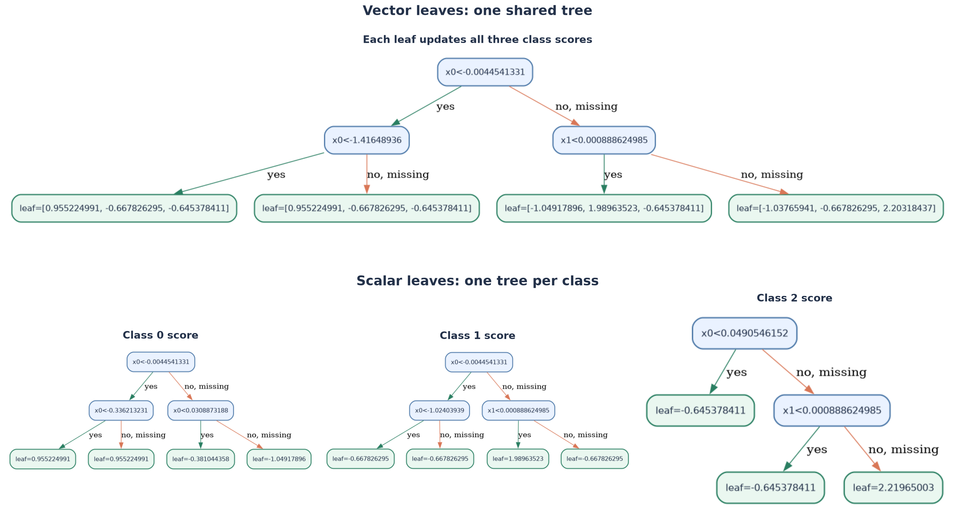
By default, XGBoost handles these problems by building one stack of scalar-leaf trees for each output. The vector-leaf model offers another choice: build one shared tree whose leaves hold a vector of predictions.
Across ten real-world multiclass datasets, vector leaves generally achieved lower held-out loss and produced simpler models. When outputs benefit from using the same splits, vector-leaf models can also train and predict faster and be less susceptible to spurious features. In this post, we explore when shared tree structure helps and what trade-offs it brings.
Getting started
In XGBoost v3.4.1, the default multi_strategy="one_output_per_tree" builds a separate
scalar-leaf tree for each class at every boosting round. Set
multi_strategy="multi_output_tree" to build one shared tree with vector-valued leaves
instead.
The hist implementation supports CPU and CUDA training, categorical splits, and
reduced-gradient training. See the multi-output
tutorial for details
and examples. Vector leaves were first prototyped for the CPU hist tree method in v2.0;
after several releases of refinement, v3.4.1 is the first feature-complete implementation
for hist.
This setting changes how the classes share model structure. Each vector leaf stores a separate score update for every class, but all classes follow the same sequence of splits that routes a row to that leaf. For a problem with 32 classes, one scalar boosting round adds 32 trees, while one vector boosting round adds a single shared tree. This difference can produce far fewer splits and a much simpler model.
Why share a tree?
Suppose a tree asks whether a pixel is dark, a playing card is an ace, or a sensor reading exceeds a threshold. In a multiclass problem, the answer may be useful to several classes at once. A vector-leaf tree asks the question once, then stores a different adjustment for every class in the resulting leaf.
This is an appealing example of Occam’s razor: when one partition of the data works as well as many separate partitions, prefer the simpler representation. It can be smaller and faster to evaluate, and the shared structure can act as a useful modeling constraint, making the model more likely to generalize well for unseen data.
The trade-off is that all outputs must use the same tree structure. This works best when they benefit from similar features and split thresholds—a property we call partition compatibility. In multiclass classification, for example, a question about whether a region of an image contains ink may help distinguish several characters at once.
Partition compatibility is not the same as target correlation. Correlation says that target values move together; it does not say that the targets need the same decision boundaries. What matters here is whether the same split questions are useful across outputs. If those questions and thresholds are largely unrelated, separate scalar trees have more freedom.
A synthetic example
To illustrate the benefit of compatible partitions, we generated a multi-output regression
problem with 32 normally distributed features. Every target combines those same set of
features with different weights and a small amount of random noise. The targets therefore
need different predictions, but they all benefit from the same basic split questions. We
generated 2^20 training rows and 2^18 test rows, then compared problems with 2, 4, 8,
16, and 32 outputs. Both strategies were trained for 128 boosting rounds. This
deliberately partition-compatible dataset is the favorable case for vector leaves.
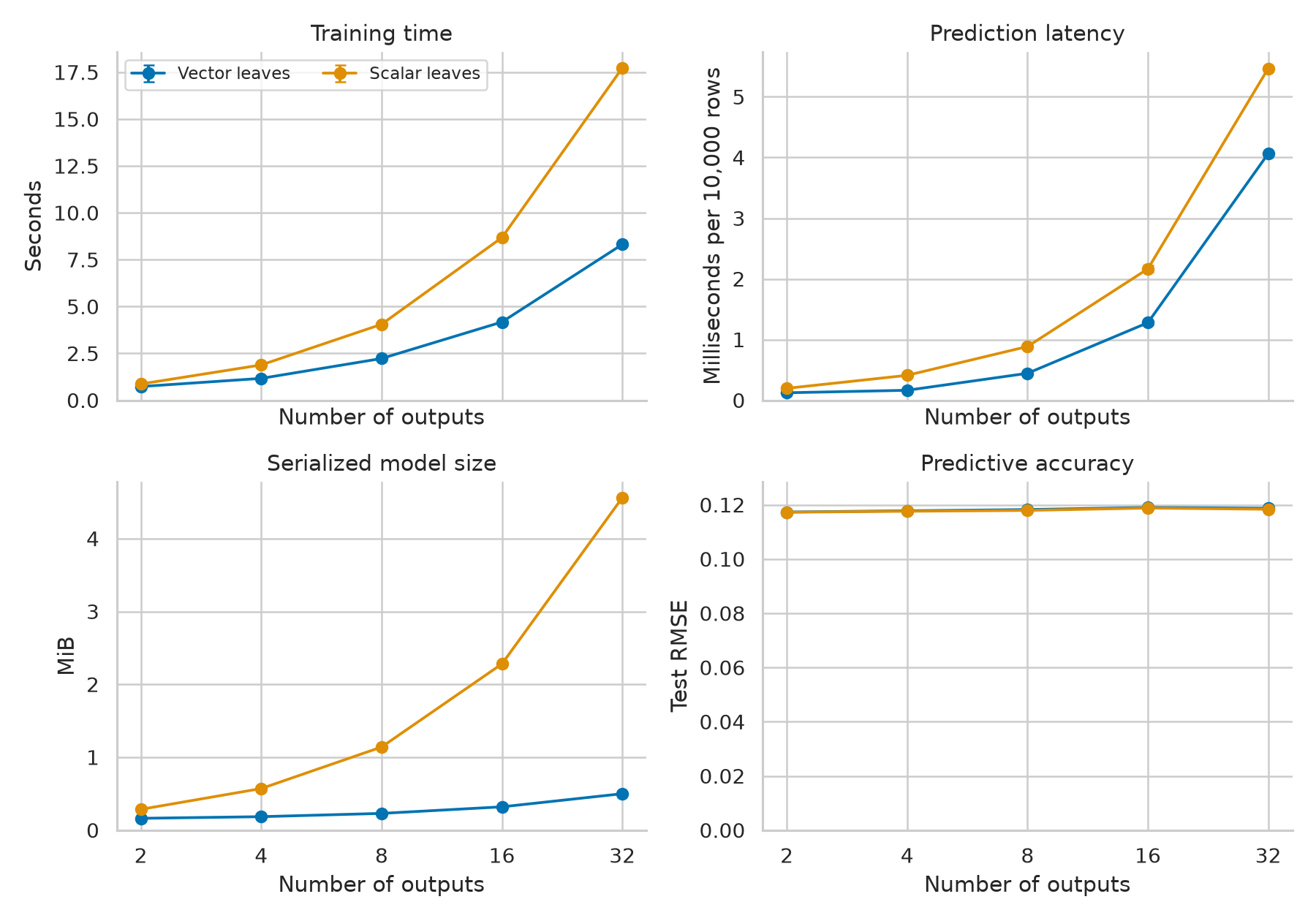
Both strategies retain essentially the same predictive error. Their complexity, however, separates as the output count grows. At 32 outputs, the vector model is about one ninth of the serialized size, and both training and prediction are faster. Separate scalar trees largely repeat the same useful structure; the vector model represents it once.
Shared partitions resist spurious features
A second controlled experiment tests the regularizing effect of sharing a tree. We generated a synthetic multiclass problem whose class probabilities come from one shared tree over a small set of signal features. Each leaf holds class-specific logits, so the true decision function is exactly partition-compatible.
We then added progressively larger sets of independent noise features. Within each paired comparison, the rows, labels, and signal stay fixed, isolating the effect of giving the models more irrelevant choices. We track how much the added noise worsens expected log loss and, from the tree dumps, how much split gain the models assign to noise.
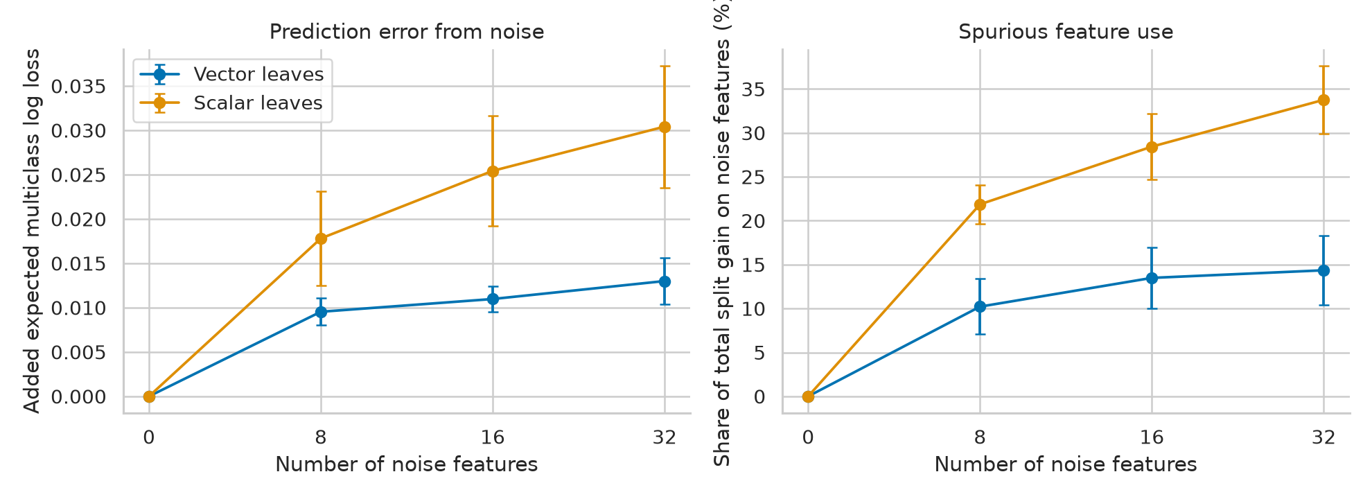
The curves separate as more distractions become available. At the largest noise setting, the scalar models devote more than twice as much split gain to irrelevant features and suffer more than twice the increase in expected log loss. A scalar class tree can promote a chance association found for one class, whereas a vector tree evaluates each split jointly across all class-score dimensions. Class-specific fluctuations therefore have less influence on the shared partition. Sharing does not eliminate noise splits, but it makes them less competitive.
What happens on real data?
We next compared the strategies on ten multiclass datasets ranging from 13,910 to more than one million rows and from 6 to 1,000 classes. The applications include forest-cover prediction, card hands, motor-drive diagnosis, gas sensing, character recognition, object recognition, and Dionis, a large tabular benchmark with 355 classes from the ChaLearn AutoML Challenge. The suite includes both balanced and heavily imbalanced class distributions.
The figure shows the selected vector model relative to the selected scalar model, with
each model selected by validation loss before the test data were evaluated. The dashed
line is parity; points to the left favor vector leaves. For example, a split ratio of
0.25 means that the vector model uses one quarter as many splits as the scalar model.
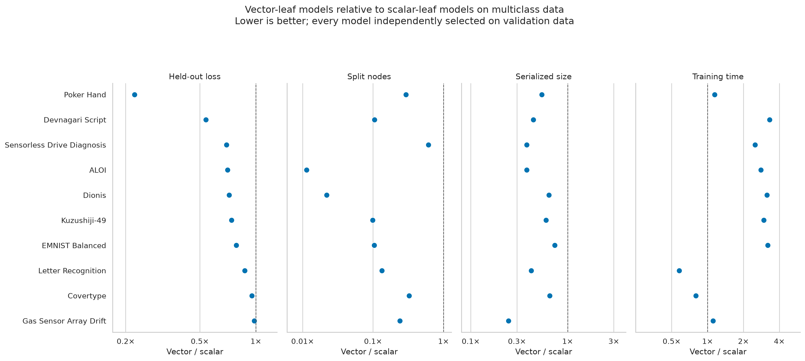
Vector leaves achieve lower held-out loss on nine of ten datasets and use fewer splits and less disk space on all ten. Poker Hand is the standout, but the pattern also appears on balanced datasets such as EMNIST and Devnagari, so class imbalance does not explain the result by itself.
Some gains come with longer training. On Devnagari, the vector model uses about three times as many boosting rounds to train. It nevertheless finishes substantially more accurate and about one third the size. Letter Recognition improves both predictive quality and training time, while Gas Sensor Drift retains a smaller advantage when trained on earlier sensor batches and evaluated on later ones. Shared structure is an advantage when it preserves enough predictive flexibility.
A practical default for multiclass classification
These results make vector leaves a strong starting point for multiclass classification,
especially as the number of classes grows. Rather than treating multi_output_tree only
as a later optimization, it is reasonable to try it first and retain a scalar model as the
comparison.
Compared with scalar models, vector models may need more boosting rounds. Each scalar round adds one tree per class, whereas each vector round adds only one shared tree. An equal round limit therefore gives the scalar model much more tree structure. On K49 and Devnagari, the vector models continued improving for substantially longer and eventually became both more accurate and smaller than their scalar counterparts.
A lower learning rate is also worth pairing with the larger round cap. XGBoost’s default learning rate is quite large. Reducing it makes each tree a smaller update and usually enables more boosting rounds. The smaller steps can make the shared, multidimensional updates easier to optimize. Dionis, for example, improved after its vector learning rate was reduced. Early stopping can then select the useful number of rounds without committing to the full cap.
About the experiments
Every real-data run used GPU histogram training and QuantileDMatrix with a DGX Spark.
Validation data controlled model selection and early stopping, and test data were
evaluated afterward. Random splits were stratified; Letter Recognition retained its
official test partition. Gas Sensor Drift used a time-ordered split because sensor
responses change over time. All these experiments use one deterministic split per dataset.
Summary
Vector leaves replace one tree per output with one shared tree whose leaves hold output-specific score updates. When outputs benefit from similar split questions, this can improve predictive quality with far fewer splits and a much smaller model, while reducing the influence of spurious features. The classification results make vector leaves a compelling default to try.
For multiclass problems, start with a generous vector boosting rounds, include a lower learning rate in the validation sweep, and let early stopping select the model. Keep the result when it provides the right balance of predictive quality, model size, and training cost for your application.